20  Eigenvectors and Eigenvalues

library(tidyverse)
library(dasc2594)
set.seed(2021)

We have just learned about change of basis in an abstract sense. Now, we will learn about a special change of basis that is “data-driven” called an eigenvector. Eigenvectors and the corresponding eigenvalues are a vital tool in data science for data compression and modeling.

Definition 20.1 An eigenvector of an \(n \times n\) matrix \(\mathbf{A}\) is a nonzero vector \(\mathbf{x}\) such that the matrix equation

\[ \begin{aligned} \mathbf{A} \mathbf{x} = \lambda \mathbf{x} \end{aligned} \]

for some scalar \(\lambda\). If there exists some \(\lambda \neq 0\) (a non-trivial solutions), then \(\lambda\) is called an eigenvalue of \(\mathbf{A}\) corresponding to the eigenvector \(\mathbf{x}\).

It is easy to check if a vector is an eigenvalue:

Let \(\mathbf{A} = \begin{pmatrix} 0 & 6 & 8 \\ 1/2 & 0 & 0 \\ 0 & 1/2 & 0 \end{pmatrix}\), \(\mathbf{u} = \begin{pmatrix} 16 \\ 4 \\ 1 \end{pmatrix}\), and \(\mathbf{v} = \begin{pmatrix} 2 \\ 2 \\ 2 \end{pmatrix}\). Determine if \(\mathbf{u}\) or \(\mathbf{v}\) are eigenvectors of \(\mathbf{A}\). If they are eigenvectors, what are the associated eigenvalues.

Here we demonstrate the eigenvector/eigenvalue relationship.

  1. If \(\mathbf{u}\) is an eigenvector of a matrix \(\mathbf{A}\), then there exists some constant \(\lambda\) such that \(\mathbf{A} \mathbf{u} = \lambda \mathbf{u}\). Checking this gives

\[ \begin{aligned} \mathbf{A} \mathbf{u} & = \begin{pmatrix} 0 & 6 & 8 \\ 1/2 & 0 & 0 \\ 0 & 1/2 & 0 \end{pmatrix} \begin{pmatrix} 16 \\ 4 \\ 1 \end{pmatrix} \\ & = \begin{pmatrix} 32 \\ 8 \\ 2 \end{pmatrix} \\ & = 2 \begin{pmatrix} 16 \\ 4 \\ 1 \end{pmatrix} \end{aligned} \]

which shows that \(\mathbf{u}\) is an eigenvector of \(\mathbf{A}\) with associated eigenvalue \(\lambda = 2\). Now, we check if \(\mathbf{v}\) is an eigenvector of \(\mathbf{A}\)

\[ \begin{aligned} \mathbf{A} \mathbf{v} & = \begin{pmatrix} 0 & 6 & 8 \\ 1/2 & 0 & 0 \\ 0 & 1/2 & 0 \end{pmatrix} \begin{pmatrix} 2 \\ 2 \\ 2 \end{pmatrix} \\ & = \begin{pmatrix} 28 \\ 1 \\ 1 \end{pmatrix} \end{aligned} \]

where there is no number \(\lambda\) such that \(\begin{pmatrix} 28 \\ 1 \\ 1 \end{pmatrix} = \lambda \begin{pmatrix} 2 \\ 2 \\ 2 \end{pmatrix}\). In R, this can be shown

A <- matrix(c(0, 1/2, 0, 6, 0, 1/2, 8, 0, 0), 3, 3)
A
     [,1] [,2] [,3]
[1,]  0.0  6.0    8
[2,]  0.5  0.0    0
[3,]  0.0  0.5    0
u <- c(16, 4, 1)
v <- c(2, 2, 2)      
# is u an eigenvector of A?
A %*% u
     [,1]
[1,]   32
[2,]    8
[3,]    2
# yes, because A %*% u = 2 u
# 2 is the eigenvalue associated with u

# is v an eigenvector of A?
A %*% v
     [,1]
[1,]   28
[2,]    1
[3,]    1
# not an eigenvectos because A %*% v is not equal to lambda * v for some lambda

Example 20.1 It is easy to check if a vector is an eigenvalue:

Let \(\mathbf{A} = \begin{pmatrix} 2 & 1 \\ 0 & 1 \end{pmatrix}\), \(\mathbf{u} = \begin{pmatrix} - \frac{\sqrt{2}}{2} \\ \frac{\sqrt{2}}{2} \end{pmatrix}\), and \(\mathbf{v} = \begin{pmatrix} 1 \\ 1 \end{pmatrix}\). Determine if \(\mathbf{u}\) or \(\mathbf{v}\) are eigenvectors of \(\mathbf{A}\). If they are eigenvectors, what are the associated eigenvalues. Now, plot \(\mathbf{u}\), \(\mathbf{A} \mathbf{u}\), \(\mathbf{v}\), and \(\mathbf{A} \mathbf{v}\) to show this relationship geometrically.

First, we determine if the vectors \(\mathbf{u}\) and \(\mathbf{v}\) are eigenvectors of \(\mathbf{A}\).

If \(\mathbf{u}\) is an eigenvector of a matrix \(\mathbf{A}\), then there exists some constant \(\lambda\) such that \(\mathbf{A} \mathbf{u} = \lambda \mathbf{u}\). Checking this gives

\[ \begin{aligned} \mathbf{A} \mathbf{u} & = \begin{pmatrix} 2 & 1 \\ 0 & 1 \end{pmatrix} \begin{pmatrix} - \frac{\sqrt{2}}{2} \\ \frac{\sqrt{2}}{2} \end{pmatrix} \\ & = \begin{pmatrix} - \frac{\sqrt{2}}{2} \\ \frac{\sqrt{2}}{2} \end{pmatrix} \end{aligned} \]

which shows that \(\mathbf{u}\) is an eigenvector of \(\mathbf{A}\) with associated eigenvalue \(\lambda = 1\). Now, we check if \(\mathbf{v}\) is an eigenvector of \(\mathbf{A}\)

\[ \begin{aligned} \mathbf{A} \mathbf{v} & = \begin{pmatrix} 2 & 1 \\ 0 & 1 \end{pmatrix} \begin{pmatrix} 1 \\ 1 \end{pmatrix} \\ & = \begin{pmatrix} 3 \\ 1 \end{pmatrix} \end{aligned} \]

where there is no number \(\lambda\) such that \(\begin{pmatrix} 3 \\ 1 \end{pmatrix} = \lambda \begin{pmatrix} 1 \\ 1 \end{pmatrix}\). In R, this can be shown

A <- matrix(c(2, 0, 1, 1), 2, 2)
u <- c(-sqrt(2)/2, sqrt(2) / 2)
v <- c(1, 1)

# is u an eigenvector of A?
A %*% u
           [,1]
[1,] -0.7071068
[2,]  0.7071068
# yes, because A %*% u = u
# 1 is the eigenvalue associated with u

# is v an eigenvector of A?
A %*% v
     [,1]
[1,]    3
[2,]    1
# not an eigenvectos because A %*% v is not equal to lambda * v for some lambda

Now, we will plot the vectors \(\mathbf{u}\) and \(\mathbf{v}\) as well as the vectors transformed by the matrix \(\mathbf{A}\) (i.e., \(\mathbf{A} \mathbf{u}\) and \(\mathbf{A} \mathbf{v}\)). The code below plot the vector \(\mathbf{u}\) in dark blue and the transformed vector \(\mathbf{A} \mathbf{u}\) in light blue. The code also plots the vector \(\mathbf{v}\) in dark red and the transformed vector \(\mathbf{A} \mathbf{v}\) in light red.

ggplot() +
    geom_segment(aes(x = 0, xend = u[1], y = 0, yend = u[2]), color = "dark blue") +
    geom_segment(aes(x = 0, xend = (A %*% u)[1], y = 0, yend = (A %*% u)[2]), color = "light blue", lty = 2) +
    geom_segment(aes(x = 0, xend = v[1], y = 0, yend = v[2]), color = "dark red") +
    geom_segment(aes(x = 0, xend = (A %*% v)[1], y = 0, yend = (A %*% v)[2]), color = "red") +
    coord_cartesian(xlim = c(-5, 5), ylim = c(-5, 5))

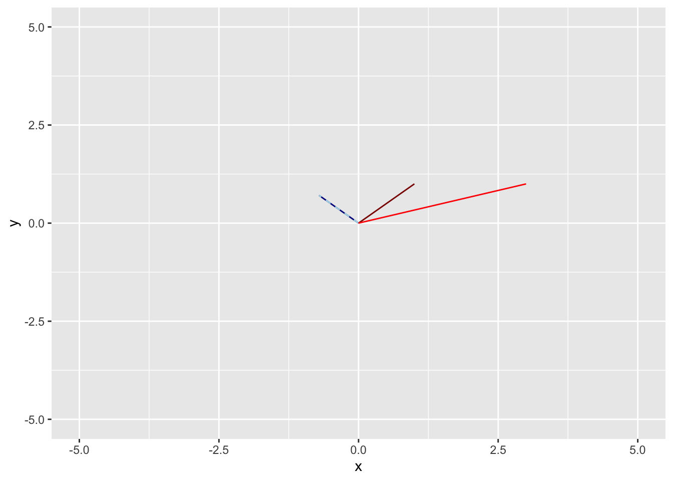
Notice that the multiplication of \(\mathbf{u}\) by \(\mathbf{A}\) gives a vector \(\mathbf{A} \mathbf{u}\) that points along the same line as \(\mathbf{u}\) because \(\mathbf{u}\) is an eigenvector of \(\mathbf{A}\). In comparison, the vector \(\mathbf{v}\) is not an eigenvector of \(\mathbf{A}\) and multiplication of \(\mathbf{v}\) by \(\mathbf{A}\) gives a vector \(\mathbf{A} \mathbf{v}\) that does not point along the same line as the vector \(\mathbf{u}\).

Example 20.2 Come up with another example and another plot that shows the similar result as the example above.

The solution (TBD)

Thus, we end up with the understanding that nn eigenvector is a (nonzero) vector \(\mathbf{x}\) that gets mapped to a scalar multiple of itself \(\lambda \mathbf{x}\) by the matrix transformation defined by \(T: \mathbf{x} \rightarrow \mathbf{A}\mathbf{x} = \mathbf{x}\). As such, when \(\mathbf{x}\) is an eigenvector of \(\mathbf{A}\) we say that \(\mathbf{x}\) and \(\mathbf{A} \mathbf{x}\) are collinear with the origin (\(\mathbf{0}\)) and each other in the sense that these points lie on the same line that goes through the origin.

Note: The matrix \(\mathbf{A}\) must be an \(n \times n\) square matrix. A similar decomposition (called the singular value decomposition) can be used for rectangular matrices.

Example 20.3 Example: reflection Draw images: https://textbooks.math.gatech.edu/ila/eigenvectors.html

Theorem 20.1 (The Distinct Eigenvalues Theorem) Let \(\mathbf{v}_1, \ldots, \mathbf{v}_n\) be eigenvectors of a matrix \(\mathbf{A}\) and suppose the corresponding eigenvalues are \(\lambda_1, \lambda_2, \ldots, \lambda_n\) are all distinct (different values). Then, the set of vectors \(\{\mathbf{v}_1, \ldots, \mathbf{v}_n\}\) is linearly independent.

Suppose the set \(\{\mathbf{v}_1, \ldots, \mathbf{v}_n\}\) is linearly dependent. Then, there is some \(j\) such that \(\mathbf{v}_j = \sum_{k = 1}^{j-1} x_k \mathbf{v}_k\). If we choose the first linearly dependent vector as \(j\), we know that the subset of vectors \(\{\mathbf{v}_1, \ldots, \mathbf{v}_{j-1}\}\) is linearly independent and

\[ \begin{aligned} \mathbf{v}_j & = x_1 \mathbf{v}_1 + \cdots x_{j-1} + \mathbf{v}_{j-1} \end{aligned} \]

for some scalars \(x_1, \ldots, x_{j-1}\). Multiplying the equation above on the left by \(\mathbf{A}\) on both sides gives

\[ \begin{aligned} \mathbf{A}\mathbf{v}_j & = \mathbf{A} (x_1 \mathbf{v}_1 + \cdots + x_{j-1} \mathbf{v}_{j-1}) \\ \lambda_j \mathbf{v}_j & = x_1 \mathbf{A} \mathbf{v}_1 + \cdots + x_{j-1} \mathbf{A} \mathbf{v}_{j-1} \\ & = x_1 \lambda_1 \mathbf{v}_1 + \cdots x_{j-1} \lambda_{j-1} + \mathbf{v}_{j-1} \\ \end{aligned} \]

Multiplying the first equation by \(\lambda_j\) and subtracting this from the second equation gives

\[ \begin{aligned} \mathbf{0} = \lambda_j \mathbf{v}_j - \lambda_j \mathbf{v}_j & = x_1 (\lambda_1 - \lambda_j) \mathbf{v}_1 + \cdots x_{j-1} + (\lambda_{j-1} - \lambda_j) \mathbf{v}_{j-1} \\ \end{aligned} \]

Because \(\lambda_k \neq \lambda_j\) for all \(k < j\), the equation above implies a linear dependence among the set of vectors \(\{\mathbf{v}_1, \ldots, \mathbf{v}_{j-1}\}\) which is a contradiction. Therefore, our assumption that there exists a linearly dependent vector \(\mathbf{v}_j\) is violated and all the \(\{\mathbf{v}_1, \ldots, \mathbf{v}_n\}\) are linearly independent.

20.1 Eigenspaces

Given a square \(n \times n\) matrix \(\mathbf{A}\), we know how to check if a given vector \(\mathbf{x}\) is an eigenvector and then how to find the eigenvalue associated with that eigenvector. Next, we want to check if a given number is an eigenvalue of \(\mathbf{A}\) and to find all the eigenvectors corresponding to that eigenvalue.

Given a square \(n \times n\) matrix \(\mathbf{A}\) and a scalar \(\lambda\), the eigenvectors of \(\mathbf{A}\) associated with the scalar \(\lambda\) (if there are eigenvectors associated with \(\lambda\)) are the nonzero solutoins to the equation \(\mathbf{A} \mathbf{x} = \lambda \mathbf{x}\). This can be written as

\[ \begin{aligned} \mathbf{A} \mathbf{x} & = \lambda \mathbf{x} \\ \mathbf{A} \mathbf{x} -\lambda \mathbf{x} & = \mathbf{0} \\ \mathbf{A} \mathbf{x} -\lambda \mathbf{I} \mathbf{x} & = \mathbf{0} \\ \left( \mathbf{A} -\lambda \mathbf{I} \right) \mathbf{x} & = \mathbf{0}. \\ \end{aligned} \]

Therefore, the eigenvectors of \(\mathbf{A}\) associated with \(\lambda\), if there are any, are the nontrivial solutions of the homogeneous matrix equation \(\left( \mathbf{A} - \lambda \mathbf{I} \right) \mathbf{x} = \mathbf{0}\). In other words, the eigenvectors are the nonzero vectors in the null space null\(\left( \mathbf{A} -\lambda \mathbf{I} \right)\). If there is not a nontrivial solution (solution \(\mathbf{x} \neq \mathbf{0}\)), then \(\lambda\) is not an eigenvalue of \(\mathbf{A}\).

Hey, we know how to find solutions to homogeneous systems of equations! Thus, we know how to find the eigenvectors of \(\mathbf{A}\). All we have to do is solve the system of linear equations \(\left( \mathbf{A} -\lambda \mathbf{I} \right) \mathbf{x} = \mathbf{0}\) for a given \(\lambda\) (actually, for all \(\lambda\)s, which we can’t do). If only there was some way to find eigenvalues \(\lambda\) (hint: there is and it is coming next chapter).

Example 20.4  

Let \(\mathbf{A} = \begin{pmatrix} 3 & 6 & -8 \\ 0 & 0 & 6 \\ 0 & 0 & 2 \end{pmatrix}\). Then an eigenvector with eigenvector \(\lambda\) is a nontrival solution to

\[ \begin{aligned} \left( \mathbf{A} - \lambda \mathbf{I} \right) \mathbf{x} & = \mathbf{0} \end{aligned} \]

which can be written as

\[ \begin{aligned} \begin{pmatrix} 3 - \lambda & 6 & -8 \\ 0 & 0 - \lambda & 6 \\ 0 & 0 & 2 - \lambda \end{pmatrix} \begin{pmatrix} x_1 \\ x_2 \\ x_3 \end{pmatrix} & = \mathbf{0} \end{aligned} \]

which can be solved for a given \(\lambda\) using an augmented matrix form and row operations to reduce to reduced row echelon form.

Letting \(\lambda = 3\), we have

\[ \begin{aligned} \begin{pmatrix} 3 - 3 & 6 & -8 \\ 0 & 0 - 3 & 6 \\ 0 & 0 & 2 - 3 \end{pmatrix} \begin{pmatrix} x_1 \\ x_2 \\ x_3 \end{pmatrix} & = \mathbf{0} \end{aligned} \]

which can be written as the matrix equation

\[ \begin{aligned} \begin{pmatrix} 0 & 6 & -8 \\ 0 & -3 & 6 \\ 0 & 0 & -1 \end{pmatrix} \begin{pmatrix} x_1 \\ x_2 \\ x_3 \end{pmatrix} & = \mathbf{0} \end{aligned} \]

Note that the columns of the matrix above are not linearly independent. Thus, we can solve a non-unique solution (the solution set is a line going through the origin) by finding the reduce row echelon form of an augmented matrix

\[ \begin{aligned} \begin{pmatrix} 0 & 6 & -8 & 0 \\ 0 & -3 & 6 & 0 \\ 0 & 0 & -1 & 0 \end{pmatrix} & \stackrel{rref}{\sim} \begin{pmatrix} 0 & 1 & 0 & 0 \\ 0 & 0 & 1 & 0 \\ 0 & 0 & 0 & 0 \end{pmatrix} \end{aligned} \]

which has solution

\[ \begin{aligned} x_1 & = x_1 \\ x_2 & = 0 \\ x_3 & = 0 \end{aligned} \]

Fixing \(x_1 = 1\) gives the eigenvector associated with \(\lambda = 3\) of \(\begin{pmatrix} 1 \\ 0 \\ 0 \end{pmatrix}\). We can verify that this is an eigenvector with matrix multiplication

\[ \begin{aligned} \begin{pmatrix} 3 & 6 & -8 \\ 0 & 0 & 6 \\ 0 & 0 & 2 \end{pmatrix} \begin{pmatrix} 1 \\ 0 \\ 0 \end{pmatrix} & = \begin{pmatrix} 3 \\ 0 \\ 0 \end{pmatrix} = 3 \begin{pmatrix} 1 \\ 0 \\ 0 \end{pmatrix} \end{aligned} \]

Using R, this can be done as

lambda <- 3
# apply rref to the augmented matrix
rref(cbind(A - lambda * diag(nrow(A)), 0))
     [,1] [,2] [,3] [,4]
[1,]    0    1    0    0
[2,]    0    0    1    0
[3,]    0    0    0    0

where the solution set is determined from the RREF form of the augmented matrix of the equation \(\left( \mathbf{A} - \lambda \mathbf{I} \right) \mathbf{x} = \mathbf{0}\)

Example 20.5  

Let \(\mathbf{A} = \begin{pmatrix} -21/5 & -34/5 & 18/5 \\ -6/5 & -14/5 & 3/5 \\ -4 & -10 & 5 \end{pmatrix}\). Find the eigenvectors associated with the eigenvalues (a) \(\lambda_1 = -4\), (b) \(\lambda_2 = 3\), and (c) \(\lambda_3 = -1\).

Given the matrix \(\mathbf{A} = \begin{pmatrix} -21/5 & -34/5 & 18/5 \\ -6/5 & -14/5 & 3/5 \\ -4 & -10 & 5 \end{pmatrix}\), we can find the eigenvectors associated with the given eigenvalues

  1. The eigenvalues associated with the first eigenvector \(\lambda_1 = -4\) by solving

\[ \begin{aligned} \left( \mathbf{A} - \lambda_1 \mathbf{I} \right) \mathbf{x} & = \mathbf{0} \end{aligned} \]

which can be written as

\[ \begin{aligned} \begin{pmatrix} -21/5 - \lambda_1 & -34/5 & 18/5 \\ -6/5 & -14/5 - \lambda_1 & 3/5 \\ -4 & -10 & 5 - \lambda_1 \end{pmatrix} \begin{pmatrix} x_1 \\ x_2 \\ x_3 \end{pmatrix} & = \mathbf{0} \end{aligned} \]

and can be solved for \(\lambda_1\) using an augmented matrix form and row operations to reduce to reduced row echelon form.

Letting \(\lambda_1 = -4\), we have

\[ \begin{aligned} \begin{pmatrix} -21/5 - -4 & -34/5 & 18/5 \\ -6/5 & -14/5 - -4 & 3/5 \\ -4 & -10 & 5 - -4 \end{pmatrix} \begin{pmatrix} x_1 \\ x_2 \\ x_3 \end{pmatrix} & = \mathbf{0} \end{aligned} \]

which results in the augmented matrix

\[ \begin{aligned} \begin{pmatrix} -1/5 & -34/5 & 18/5 & 0 \\ -6/5 & 6/5 & 3/5 & 0 \\ -4 & -10 & 9 & 0 \end{pmatrix} \end{aligned} \]

Reducing the augmented matrix to reduced row echelon form gives

\[ \begin{aligned} \begin{pmatrix} -1/5 & -34/5 & 18/5 & 0 \\ -6/5 & 6/5 & 3/5 & 0 \\ -4 & -10 & 9 & 0 \end{pmatrix} & \stackrel{rref}{\sim} \begin{pmatrix} 1 & 0 & -1 & 0 \\ 0 & 1 & -1/2 & 0 \\ 0 & 0 & 0 & 0 \end{pmatrix} \end{aligned} \]

which has solution

\[ \begin{aligned} x_1 - x_3 & = 0 \\ x_2 - \frac{1}{2} x_3 & = 0 \\ x_3 & = x_3 \end{aligned} \]

Fixing \(x_3 = 1\) gives the eigenvector associated with \(\lambda_1 = -4\) of \(\mathbf{x}_1 = \begin{pmatrix} 1 \\ 1/2 \\ 1 \end{pmatrix}\). We can verify that this is an eigenvector with matrix multiplication to show \(\mathbf{A} \mathbf{x}_1 = \lambda_1 \mathbf{x}_1\)

\[ \begin{aligned} \begin{pmatrix} -21/5 & -34/5 & 18/5 \\ -6/5 & -14/5 & 3/5 \\ -4 & -10 & 5 \end{pmatrix} \begin{pmatrix} 1 \\ 1/2 \\ 1 \end{pmatrix} & = \begin{pmatrix} -4 \\ -2 \\ -4 \end{pmatrix} = -4 \begin{pmatrix} 1 \\ 1/2 \\ 1 \end{pmatrix} \end{aligned} \]

Using R, this is

A <- matrix(c(-21/5, -6/5, -4, -34/5, -14/5, -10, 18/5,  3/5, 5), 3, 3)
lambda_1 <- -4
rref(cbind(A - lambda_1 * diag(nrow(A)), 0))
     [,1] [,2] [,3] [,4]
[1,]    1    0 -1.0    0
[2,]    0    1 -0.5    0
[3,]    0    0  0.0    0

Verifying that the eigenvalue \(\mathbf{x}_1 = \begin{pmatrix} 1 \\ 1/2 \\ 1 \end{pmatrix}\) is an eigenvector is

x_1 <- c(1, 1/2, 1)
all.equal(drop(A %*% x_1), lambda_1 * x_1) # drop() makes a matrix with one column a vector
[1] TRUE
  1. The eigenvalues associated with the second eigenvector \(\lambda_2 = 3\) by solving

\[ \begin{aligned} \left( \mathbf{A} - \lambda_2 \mathbf{I} \right) \mathbf{x} & = \mathbf{0} \end{aligned} \]

which can be written as

\[ \begin{aligned} \begin{pmatrix} -21/5 - \lambda_2 & -34/5 & 18/5 \\ -6/5 & -14/5 - \lambda_2 & 3/5 \\ -4 & -10 & 5 - \lambda_2 \end{pmatrix} \begin{pmatrix} x_1 \\ x_2 \\ x_3 \end{pmatrix} & = \mathbf{0} \end{aligned} \]

and can be solved for \(\lambda_2\) using an augmented matrix form and row operations to reduce to reduced row echelon form.

Letting \(\lambda_2 = 3\), we have

\[ \begin{aligned} \begin{pmatrix} -21/5 - 3 & -34/5 & 18/5 \\ -6/5 & -14/5 - 3 & 3/5 \\ -4 & -10 & 5 - 3 \end{pmatrix} \begin{pmatrix} x_1 \\ x_2 \\ x_3 \end{pmatrix} & = \mathbf{0} \end{aligned} \]

which results in the augmented matrix

\[ \begin{aligned} \begin{pmatrix} -36/5 & -34/5 & 18/5 & 0 \\ -6/5 & -29/5 & 3/5 & 0 \\ -4 & -10 & 2 & 0 \end{pmatrix} \end{aligned} \]

Reducing the augmented matrix to reduced row echelon form gives

\[ \begin{aligned} \begin{pmatrix} -36/5 & -34/5 & 18/5 & 0 \\ -6/5 & -29/5 & 3/5 & 0 \\ -4 & -10 & 2 & 0 \end{pmatrix} & \stackrel{rref}{\sim} \begin{pmatrix} 1 & 0 & -1/2 & 0 \\ 0 & 1 & 0 & 0 \\ 0 & 0 & 0 & 0 \end{pmatrix} \end{aligned} \]

which has solution

\[ \begin{aligned} x_1 - \frac{1}{2} x_3 & = 0 \\ x_2 & = 0 \\ x_3 & = x_3 \end{aligned} \]

Fixing \(x_3 = 1\) gives the eigenvector associated with \(\lambda_2 = 3\) of \(\mathbf{x}_2 = \begin{pmatrix} 1/2 \\ 0 \\ 1 \end{pmatrix}\). We can verify that this is an eigenvector with matrix multiplication to show \(\mathbf{A} \mathbf{x}_2 = \lambda_2 \mathbf{x}_2\)

\[ \begin{aligned} \begin{pmatrix} -21/5 & -34/5 & 18/5 \\ -6/5 & -14/5 & 3/5 \\ -4 & -10 & 5 \end{pmatrix} \begin{pmatrix} 1/2 \\ 0 \\ 1 \end{pmatrix} & = \begin{pmatrix} 3/2 \\ 0 \\ 3 \end{pmatrix} = 3 \begin{pmatrix} 1/2 \\ 0 \\ 1 \end{pmatrix} \end{aligned} \]

Using R, this is

A <- matrix(c(-21/5, -6/5, -4, -34/5, -14/5, -10, 18/5,  3/5, 5), 3, 3)
lambda_2 <- 3
rref(cbind(A - lambda_2 * diag(nrow(A)), 0))
     [,1] [,2] [,3] [,4]
[1,]    1    0 -0.5    0
[2,]    0    1  0.0    0
[3,]    0    0  0.0    0

Verifying that the eigenvalue \(\mathbf{x}_1 = \begin{pmatrix} 1 \\ 1/2 \\ 1 \end{pmatrix}\) is an eigenvector is

x_2 <- c(1/2, 0, 1)
all.equal(drop(A %*% x_2), lambda_2 * x_2) # drop() makes a matrix with one column a vector
[1] TRUE
  1. The eigenvalues associated with the third eigenvector \(\lambda_3 = -1\) by solving

\[ \begin{aligned} \left( \mathbf{A} - \lambda_3 \mathbf{I} \right) \mathbf{x} & = \mathbf{0} \end{aligned} \]

which can be written as

\[ \begin{aligned} \begin{pmatrix} -21/5 - \lambda_3 & -34/5 & 18/5 \\ -6/5 & -14/5 - \lambda_3 & 3/5 \\ -4 & -10 & 5 - \lambda_3 \end{pmatrix} \begin{pmatrix} x_1 \\ x_2 \\ x_3 \end{pmatrix} & = \mathbf{0} \end{aligned} \]

and can be solved for \(\lambda_3\) using an augmented matrix form and row operations to reduce to reduced row echelon form.

Letting \(\lambda_3 = -1\), we have

\[ \begin{aligned} \begin{pmatrix} -21/5 - -1 & -34/5 & 18/5 \\ -6/5 & -14/5 - -1 & 3/5 \\ -4 & -10 & 5 - -1 \end{pmatrix} \begin{pmatrix} x_1 \\ x_2 \\ x_3 \end{pmatrix} & = \mathbf{0} \end{aligned} \]

which results in the augmented matrix

\[ \begin{aligned} \begin{pmatrix} -16/5 & -34/5 & 18/5 & 0 \\ -6/5 & -9/5 & 3/5 & 0 \\ -4 & -10 & 6 & 0 \end{pmatrix} \end{aligned} \]

Reducing the augmented matrix to reduced row echelon form gives

\[ \begin{aligned} \begin{pmatrix} -16/5 & -34/5 & 18/5 & 0 \\ -6/5 & -9/5 & 3/5 & 0 \\ -4 & -10 & 6 & 0 \end{pmatrix} & \stackrel{rref}{\sim} \begin{pmatrix} 1 & 0 & 1 & 0 \\ 0 & 1 & -1 & 0 \\ 0 & 0 & 0 & 0 \end{pmatrix} \end{aligned} \]

which has solution

\[ \begin{aligned} x_1 + x_3 & = 0 \\ x_2 - x_3 & = 0 \\ x_3 & = x_3 \end{aligned} \]

Fixing \(x_3 = 1\) gives the eigenvector associated with \(\lambda_3 = -1\) of \(\mathbf{x}_3 = \begin{pmatrix} -1 \\ 1 \\ 1 \end{pmatrix}\). We can verify that this is an eigenvector with matrix multiplication to show \(\mathbf{A} \mathbf{x}_2 = \lambda_2 \mathbf{x}_2\)

\[ \begin{aligned} \begin{pmatrix} -21/5 & -34/5 & 18/5 \\ -6/5 & -14/5 & 3/5 \\ -4 & -10 & 5 \end{pmatrix} \begin{pmatrix} -1 \\ 1 \\ 1 \end{pmatrix} & = \begin{pmatrix} 1 \\ -1 \\ -1 \end{pmatrix} = -1 \begin{pmatrix} -1 \\ 1 \\ 1 \end{pmatrix} \end{aligned} \]

Using R, this is

A <- matrix(c(-21/5, -6/5, -4, -34/5, -14/5, -10, 18/5,  3/5, 5), 3, 3)
lambda_3 <- -1
rref(cbind(A - lambda_3 * diag(nrow(A)), 0))
     [,1] [,2] [,3] [,4]
[1,]    1    0    1    0
[2,]    0    1   -1    0
[3,]    0    0    0    0

Verifying that the eigenvalue \(\mathbf{x}_1 = \begin{pmatrix} 1 \\ 1/2 \\ 1 \end{pmatrix}\) is an eigenvector is

x_3 <- c(-1, 1, 1)
all.equal(drop(A %*% x_3), lambda_3 * x_3) # drop() makes a matrix with one column a vector
[1] TRUE

Now, let’s compare the output of the eigen() function in R to these eigenvectors calculated “by hand.” The eigen() function returns the two objects named $values that contain the eigenvalues of \(\mathbf{A}\) and the object $vectors that contains a matrix of eigenvectors as the columns fo the matrix. Each eigenvalue corresponds to the respective column of the eigenvector matrix.

eigen(A)
eigen() decomposition
$values
[1] -4  3 -1

$vectors
          [,1]          [,2]       [,3]
[1,] 0.6666667 -4.472136e-01 -0.5773503
[2,] 0.3333333 -3.041122e-16  0.5773503
[3,] 0.6666667 -8.944272e-01  0.5773503

Note that the eigenvectors returned by the eigen() function are the same as those in the example, but the vectors are different. However, the vectors from eigen() point in the same direction as those found “by hand” and only differ in the length of the vector. For example, we found the eigenvector associated with the eigenvalue -4 to be \(\begin{pmatrix} 1 \\ 1/2 \\ 1 \end{pmatrix}\) which points in the same direction as the vector from eigen() of \(\begin{pmatrix} 2/3 \\ 1/3 \\ 2/3 \end{pmatrix}\) which is just a scalar multiple of the vector found “by hand.” Recall that when we found a solution using RREF and the augmented matrix, the solution set was infinite (a line) and we just set the free variable equal to 1. Another equally valid solution would be to set the free variable so that the total length of the vector is 1, and this is what the eigen() function does.

Definition 20.2 Let \(\mathbf{A}\) be an \(n \times n\) matrix and let \(\lambda\) be an eigenvalue of \(\mathbf{A}\). Then, the \(\lambda\)-eigenspace of \(\mathbf{A}\) is the solution set of the matrix equation \(\left( \mathbf{A} - \lambda \mathbf{I} \right) \mathbf{x} = \mathbf{0}\) which is the subspace null(\(\mathbf{A} - \lambda \mathbf{I}\)).

Therefore, the \(\lambda\)-eigenspace is a subspace (the null space of any matrix is a subspace) that contains the zero vector \(\mathbf{0}\) and all the eigenvectors of \(\mathbf{A}\) with corresponding eigenvalue \(\lambda\).

Example 20.6  

For \(\lambda\) = (a) -2, (b) 1, and (c) 3, decide if \(\lambda\) is a eigenvalue of the matrix \(\mathbf{A} = \begin{pmatrix} 3 & 0 \\ -3 & 2 \end{pmatrix}\) and if so, compute a basis for the \(\lambda\)-eigenspace.

Given the matrix \(\mathbf{A}\) defined in the example, we will check if any of the values of \(\lambda\) are eigenvalues.

A <-  matrix(c(3, -3, 0, 2), 2, 2)
  1. First, we check if \(\lambda = -2\) is an eigenvalue of \(\mathbf{A}\). If \(\lambda = -2\) is an eigenvalue of \(\mathbf{A}\), then there is a non-trivial solution to

\[ \begin{aligned} \left( \mathbf{A} - \lambda\mathbf{I} \right) \mathbf{x} & = \mathbf{0} \end{aligned} \]

The homogeneous system of equations can be written as

\[ \begin{aligned} \begin{pmatrix} 3 - \lambda & 0 \\ -3 & 2 - \lambda \end{pmatrix} \begin{pmatrix} x_1 \\ x_2 \end{pmatrix} & = \mathbf{0} \end{aligned} \]

and can be solved for \(\lambda = -2\) using an augmented matrix form and row operations to reduce to reduced row echelon form where

\[ \begin{aligned} \begin{pmatrix} 3 - -2 & 0 \\ -3 & 2 - -2 \end{pmatrix} \begin{pmatrix} x_1 \\ x_2 \end{pmatrix} & = \mathbf{0} \end{aligned} \]

which results in the augmented matrix

\[ \begin{aligned} \begin{pmatrix} 5 & 0 & 0 \\ -3 & 4 & 0 \end{pmatrix} \end{aligned} \]

Reducing the augmented matrix to reduced row echelon form gives

\[ \begin{aligned} \begin{pmatrix} 5 & 0 & 0 \\ -3 & 4 & 0 \end{pmatrix} & \stackrel{rref}{\sim} \begin{pmatrix} 1 & 0 & 0 \\ 0 & 1 & 0 \end{pmatrix} \end{aligned} \]

which has solution

\[ \begin{aligned} x_1 & = 0 \\ x_2 & = 0 \end{aligned} \]

which is the trivial solution. Thus, \(\lambda = -2\) is not an eigenvalue of \(\mathbf{A}\).

Using R, this is

A <-  matrix(c(3, -3, 0, 2), 2, 2)
lambda <- -2
rref(cbind(A - lambda * diag(nrow(A)), 0))
     [,1] [,2] [,3]
[1,]    1    0    0
[2,]    0    1    0

Because there is only the trivial solution \(\mathbf{x} = \mathbf{0}\), \(\lambda = -2\) is not an eigenvalue of \(\mathbf{A}\).

lambda <- 1
  1. Next, we check if \(\lambda = 1\) is an eigenvalue of \(\mathbf{A}\). If \(\lambda = 1\) is an eigenvalue of \(\mathbf{A}\), then there is a non-trivial solution to

\[ \begin{aligned} \left( \mathbf{A} - \lambda\mathbf{I} \right) \mathbf{x} & = \mathbf{0} \end{aligned} \]

The homogeneous system of equations can be written as

\[ \begin{aligned} \begin{pmatrix} 3 - \lambda & 0 \\ -3 & 2 - \lambda \end{pmatrix} \begin{pmatrix} x_1 \\ x_2 \end{pmatrix} & = \mathbf{0} \end{aligned} \]

and can be solved for \(\lambda = 1\) using an augmented matrix form and row operations to reduce to reduced row echelon form where

\[ \begin{aligned} \begin{pmatrix} 3 - 1 & 0 \\ -3 & 2 - 1 \end{pmatrix} \begin{pmatrix} x_1 \\ x_2 \end{pmatrix} & = \mathbf{0} \end{aligned} \]

which results in the augmented matrix

\[ \begin{aligned} \begin{pmatrix} 2 & 0 & 0 \\ -3 & 1 & 0 \end{pmatrix} \end{aligned} \]

Reducing the augmented matrix to reduced row echelon form gives

\[ \begin{aligned} \begin{pmatrix} 2 & 0 & 0 \\ -3 & 1 & 0 \end{pmatrix} & \stackrel{rref}{\sim} \begin{pmatrix} 1 & 0 & 0 \\ 0 & 1 & 0 \end{pmatrix} \end{aligned} \]

which has solution

\[ \begin{aligned} x_1 & = 0 \\ x_2 & = 0 \end{aligned} \]

which is the trivial solution. Thus, \(\lambda = 1\) is not an eigenvalue of \(\mathbf{A}\).

Fixing \(x_3 = 1\) gives the eigenvector associated with \(\lambda_3 = NA\) of \(\mathbf{x}_3 = \begin{pmatrix} -1 \\ 1 \\ 1 \end{pmatrix}\). We can verify that this is an eigenvector with matrix multiplication to show \(\mathbf{A} \mathbf{x}_2 = \lambda_2 \mathbf{x}_2\)

\[ \begin{aligned} \begin{pmatrix} 3 & 0 \\ -3 & 2 \end{pmatrix} \begin{pmatrix} -1 \\ 1 \end{pmatrix} & = \begin{pmatrix} -3 \\ 5 \end{pmatrix} = 1 \begin{pmatrix} -1 \\ 1 \end{pmatrix} \end{aligned} \]

Using R, this is

A <-  matrix(c(3, -3, 0, 2), 2, 2)
lambda <- 1
rref(cbind(A - lambda * diag(nrow(A)), 0))
     [,1] [,2] [,3]
[1,]    1    0    0
[2,]    0    1    0

Because there is only the trivial solution \(\mathbf{x} = \mathbf{0}\), \(\lambda = 1\) is not an eigenvalue of \(\mathbf{A}\).

lambda <- 3
  1. Next, we check if \(\lambda = 3\) is an eigenvalue of \(\mathbf{A}\). If \(\lambda = 3\) is an eigenvalue of \(\mathbf{A}\), then there is a non-trivial solution to

\[ \begin{aligned} \left( \mathbf{A} - \lambda\mathbf{I} \right) \mathbf{x} & = \mathbf{0} \end{aligned} \]

The homogeneous system of equations can be written as

\[ \begin{aligned} \begin{pmatrix} 3 - \lambda & 0 \\ -3 & 2 - \lambda \end{pmatrix} \begin{pmatrix} x_1 \\ x_2 \end{pmatrix} & = \mathbf{0} \end{aligned} \]

and can be solved for \(\lambda = 3\) using an augmented matrix form and row operations to reduce to reduced row echelon form where

\[ \begin{aligned} \begin{pmatrix} 3 - 3 & 0 \\ -3 & 2 - 3 \end{pmatrix} \begin{pmatrix} x_1 \\ x_2 \end{pmatrix} & = \mathbf{0} \end{aligned} \]

which results in the augmented matrix

\[ \begin{aligned} \begin{pmatrix} 0 & 0 & 0 \\ -3 & -1 & 0 \end{pmatrix} \end{aligned} \]

Reducing the augmented matrix to reduced row echelon form gives

\[ \begin{aligned} \begin{pmatrix} 0 & 0 & 0 \\ -3 & -1 & 0 \end{pmatrix} & \stackrel{rref}{\sim} \begin{pmatrix} 1 & 1/3 & 0 \\ 0 & 0 & 0 \end{pmatrix} \end{aligned} \]

which has solution

\[ \begin{aligned} x_1 + \frac{1}{3} x_2 & = 0 \\ x_2 & = x_2 \end{aligned} \]

where the solution can be chosen by setting \(x_2 = 1\) giving the eigenvector associated with \(\lambda = 3\) of \(\mathbf{x} = \begin{pmatrix} -1/3 \\ 1 \end{pmatrix}\). We can verify that this is an eigenvector with matrix multiplication to show \(\mathbf{A} \mathbf{x} = \lambda \mathbf{x}\)

\[ \begin{aligned} \begin{pmatrix} 3 & 0 \\ -3 & 2 \end{pmatrix} \begin{pmatrix} -1/3 \\ 1 \end{pmatrix} & = \begin{pmatrix} -1 \\ 3 \end{pmatrix} = 3 \begin{pmatrix} -1/3 \\ 1 \end{pmatrix} \end{aligned} \]

Using R, this is

A <-  matrix(c(3, -3, 0, 2), 2, 2)
lambda <- 3
rref(cbind(A - lambda * diag(nrow(A)), 0))
     [,1]      [,2] [,3]
[1,]    1 0.3333333    0
[2,]    0 0.0000000    0

Verifying that the eigenvalue \(\mathbf{x} = \begin{pmatrix} -1/3 \\ 1 \end{pmatrix}\) is an eigenvector is

x <- c(-1/3, 1)
all.equal(drop(A %*% x), lambda * x) # drop() makes a matrix with one column a vector
[1] TRUE

Now, because we know that \(\lambda = 3\) is an eigenvalue of \(\mathbf{A}\) and the homogeneous system of equations \(\left(\mathbf{A} - \lambda \mathbf{I} \right) \mathbf{x} = \mathbf{0}\) has a unique solution, the vector \(\begin{pmatrix} -1/3 \\ 1 \end{pmatrix}\) forms a basis for the 3-eigenspace of \(\mathbf{A}\).

Example 20.7  

Let \(\mathbf{A} = \begin{pmatrix} 17/5 & 8/5 & -6/5 \\ 0 & 3 & 0 \\ 4/5 & 16/5 & 3/5 \end{pmatrix}\). Find the eigenvectors associated with the eigenvalues (a) \(\lambda = 3\) and (b) \(\lambda = 1\). For each eigen value, also find the basis for the associated eigen-space.

Given the matrix \(\mathbf{A} = \begin{pmatrix} 17/5 & 8/5 & -6/5 \\ 0 & 3 & 0 \\ 4/5 & 16/5 & 3/5 \end{pmatrix}\), we can find the eigenvectors associated with the given eigenvalues

  1. The eigenvalues associated with the first eigenvector \(\lambda = 3\) by solving

\[ \begin{aligned} \left( \mathbf{A} - \lambda \mathbf{I} \right) \mathbf{x} & = \mathbf{0} \end{aligned} \]

which can be written as

\[ \begin{aligned} \begin{pmatrix} 17/5 - \lambda & 8/5 & -6/5 \\ 0 & 3 - \lambda & 0 \\ 4/5 & 16/5 & 3/5 - \lambda \end{pmatrix} \begin{pmatrix} x_1 \\ x_2 \\ x_3 \end{pmatrix} & = \mathbf{0} \end{aligned} \]

and can be solved for \(\lambda\) using an augmented matrix form and row operations to reduce to reduced row echelon form.

Letting \(\lambda = 3\), we have

\[ \begin{aligned} \begin{pmatrix} 17/5 - 3 & 8/5 & -6/5 \\ 0 & 3 - 3 & 0 \\ 4/5 & 16/5 & 3/5 - 3 \end{pmatrix} \begin{pmatrix} x_1 \\ x_2 \\ x_3 \end{pmatrix} & = \mathbf{0} \end{aligned} \]

which results in the augmented matrix

\[ \begin{aligned} \begin{pmatrix} 2/5 & 8/5 & -6/5 & 0 \\ 0 & 0 & 0 & 0 \\ 4/5 & 16/5 & -12/5 & 0 \end{pmatrix} \end{aligned} \]

Reducing the augmented matrix to reduced row echelon form gives

\[ \begin{aligned} \begin{pmatrix} 2/5 & 8/5 & -6/5 & 0 \\ 0 & 0 & 0 & 0 \\ 4/5 & 16/5 & -12/5 & 0 \end{pmatrix} & \stackrel{rref}{\sim} \begin{pmatrix} 1 & 4 & -3 & 0 \\ 0 & 0 & 0 & 0 \\ 0 & 0 & 0 & 0 \end{pmatrix} \end{aligned} \]

which has solution

\[ \begin{aligned} x_1 + 4 x_2 - x_33 & = 0 \\ x_2 & = x_2 \\ x_3 & = x_3 \end{aligned} \]

Where there are two free variables which suggests that the dimension of the solution space is 2 (the solution set defines a plane and will have 2 basis vectors. Fixing \(x_2 = 1\) and \(x_3 = 0\) gives the first eigenvector associated with \(\lambda = 3\) of \(\mathbf{x}_1 = \begin{pmatrix} -4 \\ 1 \\ 0 \end{pmatrix}\). We can verify that this is an eigenvector with matrix multiplication to show \(\mathbf{A} \mathbf{x}_1 = \lambda \mathbf{x}_1\)

\[ \begin{aligned} \begin{pmatrix} 17/5 & 8/5 & -6/5 \\ 0 & 3 & 0 \\ 4/5 & 16/5 & 3/5 \end{pmatrix} \begin{pmatrix} -4 \\ 1 \\ 0 \end{pmatrix} & = \begin{pmatrix} -12 \\ 3 \\ 0 \end{pmatrix} = 3 \begin{pmatrix} -4 \\ 1 \\ 0 \end{pmatrix} \end{aligned} \]

The second basis vector for the eigenspace associated with \(\lambda = 3\) can be found by fixing \(x_2 = 0\) and \(x_3 = 1\) to get the eigenvector \(\mathbf{x}_2 = \begin{pmatrix} 3 \\ 0 \\ 1 \end{pmatrix}\). We can verify that this is an eigenvector with matrix multiplication to show \(\mathbf{A} \mathbf{x}_2 = \lambda \mathbf{x}_2\)

\[ \begin{aligned} \begin{pmatrix} 17/5 & 8/5 & -6/5 \\ 0 & 3 & 0 \\ 4/5 & 16/5 & 3/5 \end{pmatrix} \begin{pmatrix} 3 \\ 0 \\ 1 \end{pmatrix} & = \begin{pmatrix} 9 \\ 0 \\ 3 \end{pmatrix} = 3 \begin{pmatrix} 3 \\ 0 \\ 1 \end{pmatrix} \end{aligned} \]

Thus, the basis for 3-eigenspace is \(\left\{ \begin{pmatrix} -4 \\ 1 \\ 0 \end{pmatrix}, \begin{pmatrix} 3 \\ 0 \\ 1 \end{pmatrix}\right\}\). Note that this is the same as finding a basis for the null space of \(\left(\mathbf{A} - \lambda \mathbf{I} \right)\).

Using R, this is

A <- matrix(c(17/5, 0, 4/5, 8/5, 3, 16/5, -6/5, 0, 3/5), 3, 3)
lambda <- 3
rref(cbind(A - lambda * diag(nrow(A)), 0))
     [,1] [,2] [,3] [,4]
[1,]    1    4   -3    0
[2,]    0    0    0    0
[3,]    0    0    0    0

Verifying that the eigenvalue \(\mathbf{x}_1 = \begin{pmatrix} -4 \\ 1 \\ 0 \end{pmatrix}\) is an eigenvector and that \(\mathbf{x}_2 = \begin{pmatrix} 3 \\ 0 \\ 1 \end{pmatrix}\) is an eigenvector

x_1 <- c(-4, 1, 0)
all.equal(drop(A %*% x_1), lambda * x_1) # drop() makes a matrix with one column a vector
[1] TRUE
x_2 <- c(3, 0, 1)
all.equal(drop(A %*% x_2), lambda * x_2) # drop() makes a matrix with one column a vector
[1] TRUE
lambda <- 1
  1. The eigenvalues associated with the second eigenvector \(\lambda = 1\) by solving

\[ \begin{aligned} \left( \mathbf{A} - \lambda \mathbf{I} \right) \mathbf{x} & = \mathbf{0} \end{aligned} \]

which can be written as

\[ \begin{aligned} \begin{pmatrix} 17/5 - \lambda & 8/5 & -6/5 \\ 0 & 3 - \lambda & 0 \\ 4/5 & 16/5 & 3/5 - \lambda \end{pmatrix} \begin{pmatrix} x_1 \\ x_2 \\ x_3 \end{pmatrix} & = \mathbf{0} \end{aligned} \]

and can be solved for \(\lambda\) using an augmented matrix form and row operations to reduce to reduced row echelon form.

Letting \(\lambda = 1\), we have

\[ \begin{aligned} \begin{pmatrix} 17/5 - 1 & 8/5 & -6/5 \\ 0 & 3 - 1 & 0 \\ 4/5 & 16/5 & 3/5 - 1 \end{pmatrix} \begin{pmatrix} x_1 \\ x_2 \\ x_3 \end{pmatrix} & = \mathbf{0} \end{aligned} \]

which results in the augmented matrix

\[ \begin{aligned} \begin{pmatrix} 12/5 & 8/5 & -6/5 & 0 \\ 0 & 2 & 0 & 0 \\ 4/5 & 16/5 & -2/5 & 0 \end{pmatrix} \end{aligned} \]

Reducing the augmented matrix to reduced row echelon form gives

\[ \begin{aligned} \begin{pmatrix} 12/5 & 8/5 & -6/5 & 0 \\ 0 & 2 & 0 & 0 \\ 4/5 & 16/5 & -2/5 & 0 \end{pmatrix} & \stackrel{rref}{\sim} \begin{pmatrix} 1 & 0 & -1/2 & 0 \\ 0 & 1 & 0 & 0 \\ 0 & 0 & 0 & 0 \end{pmatrix} \end{aligned} \]

which has solution

\[ \begin{aligned} x_1 - \frac{1}{2} x_3 & = 0 \\ x_2 & = 0 \\ x_3 & = x_3 \end{aligned} \]

Fixing \(x_3 = 1\) gives the eigenvector associated with \(\lambda= 1\) of \(\mathbf{x} = \begin{pmatrix} 1/2 \\ 0 \\ 1 \end{pmatrix}\). We can verify that this is an eigenvector associated with eigenvalue \(\lambda = 1\) with matrix multiplication to show \(\mathbf{A} \mathbf{x} = \lambda \mathbf{x}\)

\[ \begin{aligned} \begin{pmatrix} 17/5 & 8/5 & -6/5 \\ 0 & 3 & 0 \\ 4/5 & 16/5 & 3/5 \end{pmatrix} \begin{pmatrix} 1/2 \\ 0 \\ 1 \end{pmatrix} & = \begin{pmatrix} 1/2 \\ 0 \\ 1 \end{pmatrix} = NA \begin{pmatrix} 1/2 \\ 0 \\ 1 \end{pmatrix} \end{aligned} \]

Therefore, a basis for the 1-eigenspace is \(\left\{ \begin{pmatrix} 1/2 \\ 0 \\ 1 \end{pmatrix} \right\}\)

Using R, this is

A <- matrix(c(17/5, 0, 4/5, 8/5, 3, 16/5, -6/5, 0, 3/5), 3, 3)
lambda <- 1
rref(cbind(A - lambda * diag(nrow(A)), 0))
     [,1] [,2] [,3] [,4]
[1,]    1    0 -0.5    0
[2,]    0    1  0.0    0
[3,]    0    0  0.0    0

Verifying that the eigenvalue \(\mathbf{x} = \begin{pmatrix} 1 \\ 1/2 \\ 1 \end{pmatrix}\) is an eigenvector associated with eigenvalue \(\lambda = 1\) is

x <- c(1/2, 0, 1)
all.equal(drop(A %*% x), lambda * x) # drop() makes a matrix with one column a vector
[1] TRUE

20.1.1 Computing Eigenspaces

Let \(\mathbf{A}\) be a \(n \times n\) matrix and let \(\lambda\) be a scalar.

  1. \(\lambda\) is an eigenvalue of \(\mathbf{A}\) if and only if \((\mathbf{A} - \lambda \mathbf{I})\mathbf{x} = \mathbf{0}\) has a non-trivial solution. The matrix equation \((\mathbf{A} - \lambda \mathbf{I})\mathbf{x} = \mathbf{0}\) has a non-trivial solution if and only if null\((\mathbf{A} - \lambda \mathbf{I}) \neq \{\mathbf{0} \}\)

  2. Finding a basis for the \(\lambda\)-eigenspace of \(\mathbf{A}\) is equivalent to finding a basis for null\((\mathbf{A} - \lambda \mathbf{I})\) which can be done by finding parametric forms of the solutions of the homogeneous system of equations \((\mathbf{A} - \lambda \mathbf{I})\mathbf{x} = \mathbf{0}\).

  3. The dimension of the \(\lambda\)-eigenspace of \(\mathbf{A}\) is equal to the number of free variables in the system of equations \((\mathbf{A} - \lambda \mathbf{I})\mathbf{x} = \mathbf{0}\) which is the number of non-pivot columns of \(\mathbf{A} - \lambda \mathbf{I}\).

  4. The eigenvectors with eigenvalue \(\lambda\) are the nonzero vectors in null\((\mathbf{A} - \lambda \mathbf{I})\) which are equivalent to the nontrivial solutions of \((\mathbf{A} - \lambda \mathbf{I})\mathbf{x} = \mathbf{0}\).

Note that this leads of a fact about the \(0\)-eigenspace.

Definition 20.3 Let \(\mathbf{A}\) be an \(n \times n\) matrix. Then

  1. The number 0 is an eigenvalue of \(\mathbf{A}\) if and only if \(\mathbf{A}\) is not invertible.

  2. If 0 is an eigenvalue of \(\mathbf{A}\), then the 0-eigenspace of \(\mathbf{A}\) is null\((\mathbf{A})\).

0 is an eigenvalue of \(\mathbf{A}\) if and only if null\((\mathbf{A} - 0 \mathbf{I})\) = null\((\mathbf{A})\). By the invertible matrix theorem, \(\mathbf{A}\) is invertible if and only if null\((\mathbf{A}) = \{\mathbf{0}\}\) but we know that the 0-eigenspace of \(\mathbf{A}\) is not the trivial set \(\{\mathbf{0}\}\) because 0 is an eigenvalue.

Theorem 20.2 (Invertible Matrix Theorm + eigenspaces) This is an extension of the prior statement of the invertible matrix Theorem 9.5 Let \(\mathbf{A}\) be an \(n \times n\) matrix and \(T: \mathcal{R}^n \rightarrow \mathcal{R}^n\) be the linear transformation given by \(T(\mathbf{x}) = \mathbf{A}\mathbf{x}\). Then the following statements are equivalent (i.e., they are all either simultaneously true or false).

  1. \(\mathbf{A}\) is invertible.

  2. \(\mathbf{A}\) has n pivot columns.

  3. null\((\mathbf{A}) = \{\mathbf{0}\}\).

  4. The columns of \(\mathbf{A}\) are linearly independent.

  5. The columns of \(\mathbf{A}\) span \(\mathcal{R}^n\).

  6. The matrix equation \(\mathbf{A} \mathbf{x} = \mathbf{b}\) has a uniqu solution for each \(\mathbf{b} \in \mathcal{R}^n\).

  7. The transormation \(T\) is invertible.

  8. The transormation \(T\) is one-to-one.

  9. The transormation \(T\) is onto.

  10. det\((\mathbf{A}) \neq 0\)

  11. 0 is not an eigenvalue of \(\mathbf{A}\)